Simulation of Arctic Weather with a Single-Column Model

Among the various climate regimes of Earth the Arctic presents particular challenges. Complex feedback mechanisms of the ocean-ice-atmosphere system, in conjunction with the paucity of observational data, pose modeling difficulties not encountered elsewhere on the planet (Randall et al.,1998) In this study, we explore some of these issues by simulation of the Arctic environment with the Colorado State University (CSU) Single-Column Model (SCM), which is then compared with observational data gathered at the Surface Heat Budget of the Arctic (SHEBA; Moritz et al. 1993) field project. Within the context of SHEBA, observational data were provided by both the Atmospheric Radiation Measurement (ARM; DOE, 1996) program, and the First ISCCP Regional Experiment (FIRE; Randall et al. 1995; ISCCP is the International Satellite Cloud Climatology Program).

II Model and Forcing

The SCM, as the name implies, is a single grid column extracted from the CSU General Circulation Model (GCM). It has 17 layers, using generalized sigma coordinates, and the complete GCM physics package. Since it is a single grid column, however, there is no communication with adjacent grid cells and thus the SCM must be "driven" with observational data that includes dynamical fields such as advective tendencies of temperature and moisture. Observational data of this caliber is not yet available from the Arctic, so the fields of total advective tendency and surface fluxes necessary to drive the SCM were obtained from analyses generated at the European Center for Medium-Range Forecasting (ECMWF), corresponding to the location of the SHEBA site. Twice-daily soundings and routine surface observations of pressure, wind, temperature and humidity taken from the ice camp were assimilated into the ECMWF model during each analysis cycle. The data represent a model grid column approximately 60 km wide in proximity to the SHEBA ice camp, and the column position was frequently updated to account for camp drift.

**May 1998 SHEBA Ship Weather Overview**
Sunday	Monday	Tuesday	Wednesday	Thursday	Friday	Saturday
					1 low NW winds W-SW overcast light snow	2
3	4 St, As, Ci light snow	5	6	7 thin PBL St	8 high moving N winds E clouds incr snow	9
10	11 low moving N winds SW St, As, Ci snow	12	13	14 snow ends	15 High N; low S winds E PBL St thins	16
17	18 PBL St, thin Ci	19 thin PBL St, Ci	20 clear	21 thin PBL St, Ci	22 thin St	23 some As, Ci
24 clear	25 clouds incr	26	27 overcast	28 low moving N winds S-SW As, Ci drizzle	29 temps > 0 St, Ci rain	30 PBL St, As

Table 1. Weather was mainly overcast with light snow each day from 1-14 May; clouds were then variable for remainder of month with clear skies reported on 20 and 24 May; clouds increased 28-30 May with liquid precipitation reported for first time that year.

III Results

For all results presented here, total advective tendency forcing was used to drive the SCM. Figure 1 shows a time-height (pressure) time series of the moisture (left side) and temperature (right side) profiles. The top panel in each case shows the ECMWF analysis for the period, the middle panels present the SCM output, and the bottom panels are difference plots between the SCM and the ECMWF profiles. Focussing first on the temperature series, we see that the general features represented in the ECMWF analysis are also captured in the SCM output, notably the three instances of warming that occurred from days 10-12, 16-18, and 22-29. The trends in the upper troposphere above 400 mb are also in general agreement between the two models. However, inspection of the difference plot reveals a couple of marked discrepancies. In particular, the SCM tends to be warmer than the ECMWF in the lower troposphere below 400 mb by as much as 13 K in the first 10 days of the period. By contrast, between days 26-28 the SCM is colder than the ECMWF analysis by 7 K from 900 to 800 mb. Moreover, the SCM shows a cold bias in the upper troposphere above 300 mb throughout the entire period.

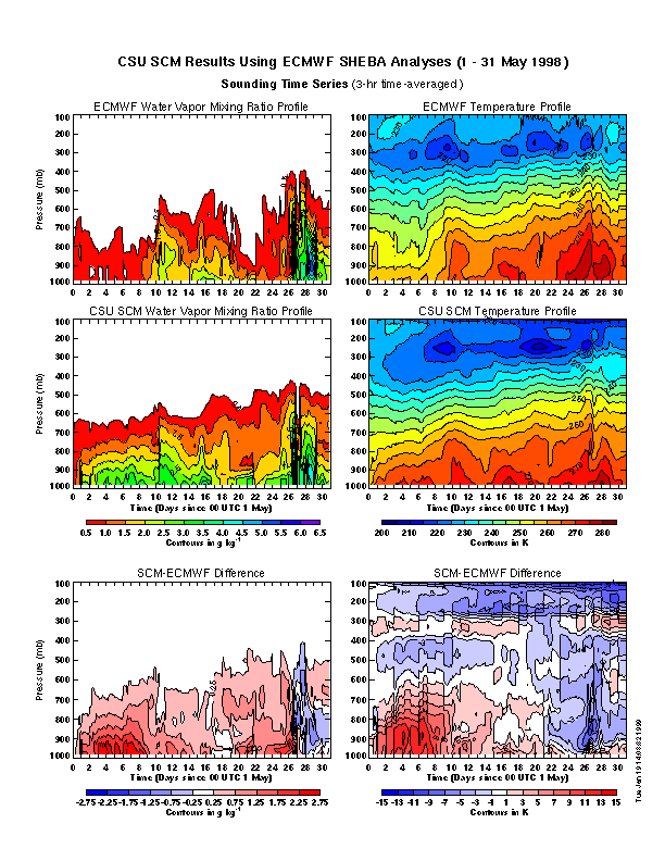
Figure 1. Time-height (pressure) plot showing time series sounding profiles of water vapor mixing ratio (left) and temperature (right). ECMWF analyses are top panels, SCM output are middle panels, and difference plots are bottom panels.

On the left side of Figure 1, we note that, as with the temperature plots, the general features of the water vapor mixing ratio profiles are discernible in both the ECMWF analysis and the SCM output. In particular, there is agreement on episodes of moistening and drying that occurred between days 10-12, 14-18, and especially 26-29. Once again, however, the difference plot reveals that there was less than complete harmony: in the first 10 days of the run the SCM is considerably more moist than the ECMWF analysis, from the surface up to 800 mb. This period corresponds to the warm bias that the SCM exhibited in the temperature profile. Similarly, towards the end of the period when the SCM showed a cold bias in the temperature profile, it also produced a dry bias compared to the ECMWF analysis. Generally, the SCM moisture appears to consistently reach higher in the lower troposphere (500 - 600 mb) than in the ECMWF analysis (500 - 700 mb).

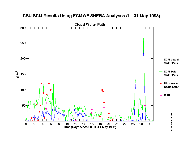
Figure 2. Time-series plot of observed versus SCM-produced cloud liquid and total cloud water path.

Figures 3 and 4 show surface net shortwave flux, and surface downwelling longwave flux, respectively. ECMWF radiative flux analyses are also shown in each for comparison. Figure 3 indicates that both the SCM and the ECMWF models consistently overestimate the net solar surface flux as observed by the 20-m tower, in some instances by over 100 W m-2. In other words, too much shortwave radiation is being absorbed at the surface which implies an incorrect determination of albedo in the SCM. Indeed, the albedo for this period as calculated by the CSU SCM averages to about 0.6 whereas the observed values were in the 0.7-0.8 range (Judy Curry, 5th Conference on Polar Meteorology and Oceanography, 79th AMS Annual Meeting, Dallas, TX, 1999).

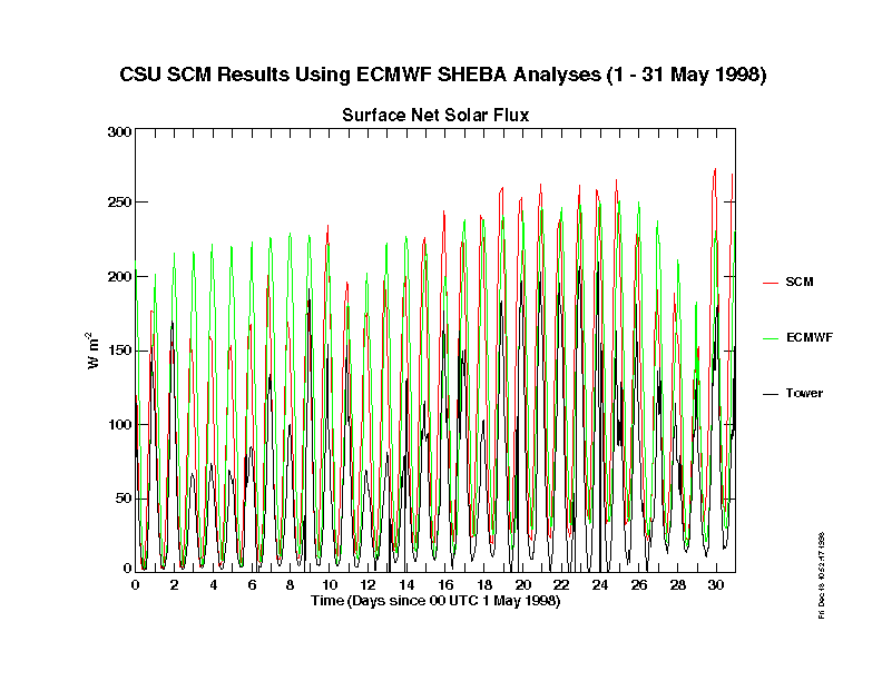
Figure 3. Time-series plot of observed versus SCM-produced and ECMWF-analyzed surface net shortwave flux.

Turning to the surface downwelling longwave flux in Figure 4, the SCM exhibits fairly good agreement with observations taken at the 20-m NOAA/ETL tower during days 9-14 and again from days 22-28. Apart from these intervals, the SCM either consistently overestimates or underestimates the flux, though paralleling the observed trends. The ECMWF model output compares more favorably with the observations throughout, as would be expected with data assimilation.

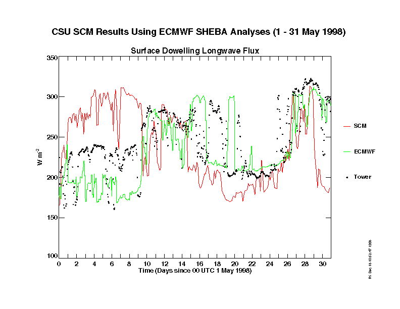
Figure 4. Time-series plot of observed versus SCM-produced and ECMWF-analyzed surface downwelling longwave flux.

The SCM's difficulty in correctly determining the surface downwelling flux could possibly be explained by deficiencies in the model's radiation parameterization. To investigate whether this might be the case, we ran several off-line tests in which the performance of the current SCM radiation parameterization was compared to that of a new parameterization being developed by Graeme Stevens' group at CSU. The results of our study are shown in Figure 5. Each of the three panels represents a different set of sounding data used as input to drive the radiation codes off-line in clear-sky mode. In the top panel, the temperature and moisture profiles as provided by the ECMWF analyses for the month of May 1998 at the SHEBA site was used as input to the codes. The second panel shows the results of using the sounding data as produced by the SCM in total advective forcing mode to drive the radiation codes. The last panel is similar to the second, only the input soundings were produced by the SCM running in relaxation mode (i.e. the model was relaxed to upstream values of temperature and moisture at each timestep). In each panel, the results produced by driving the current SCM radiation parameterization off-line are shown by the green curve (CSU 1) and those produced with the new radiation code by the blue curve (CSU 2). The red curve is identical in all three panels, and represents the ECMWF all-sky fluxes. As such, it includes the effects of clouds and is included here for comparison to the off-line clear-sky fluxes. The only regions where all three curves would be expected to agree closely would be during relatively cloudless periods, such as from days 20-26. In all three panels, we see that the CSU1 and CSU 2 curves agree very closely with each other. Further, comparing the top and bottom panels we see that the variations of the CSU 1 and CSU 2 curves are virtually identical between the two cases, whereas they differ considerably with the CSU1 and CSU 2 curves in the middle panel. Since in relaxation mode the SCM is required to relax towards upstream sounding profiles, we would expect the off-line results to be virtually identical to those driven with "observed" (ECMWF) soundings. The fact that the off-line curves are so similar to each other in each of the three sounding cases implies that the two independent radiation codes are not faulty, but rather behaving, we presume, correctly. On the other hand, the fact that the off-line results are so different in the middle panel (input sounding produced by total advective forcing) compared with those produced by either of the other input soundings suggests that it is errors produced in the temperature and moisture profiles by the SCM itself that is to blame for the discrepancy. Indeed, as can be seen in the difference plots (Figure 1), the SCM reveals considerable biases in the soundings it produced.

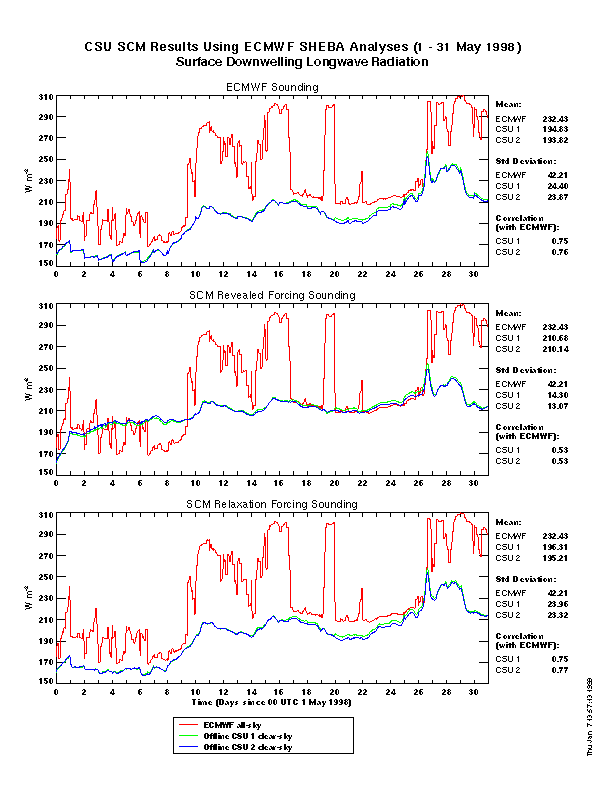
Figure 5. Time-series plots of clear-sky surface downwelling longwave radiation produced by CSU radiation parameterizations driven off-line with three different sounding data as input. ECMWF all-sky fluxes are included in each case for comparison.

IV Conclusions

The CSU SCM has been used to simulate the observed sequence of weather events for the month of May at the SHEBA site. The results show periods of both agreement and disagreement with temperature and moisture sounding analyses provided by ECMWF, as well as the in-situ moisture and radiation measurements provided by SHEBA. Additionally, though not presented here, the SCM produced more precipitation than indicated by the ECMWF analyses. The most likely causes for the discrepancies in the SCM's performance are errors arising from the parameterizations of cloud characteristics and formation processes inherited from the parent GCM. For example, inadequacies in the parameterizations of the radiation flux or cloud microphysical and optical properties, or cloud formation processes, or even the surface albedo could combine cumulatively to adversely affect the shortwave radiation received at the surface, which in turn will affect the evaluation of prognostic variables. Initially, deficiencies with atmospheric radiative transfer parameterizations were suspected as partially to blame for the mixed results in the longwave radiation fields produced by the SCM. However, as a result of the off-line tests involving the radiation codes discussed above, we are inclined to suspect the fault lies elsewhere at this time. Problems with the albedo prescription would almost certainly explain the large discrepancies between the observed and SCM-produced net surface shortwave fluxes leading to the warm bias noted at the surface. Though it would be difficult to detect the effects of changing a particular parameterization in a GCM given the complex interactions among its constituents, the SCM provides a means by which an individual parameterization made be studied in isolation. The preliminary results presented here are thus a first step in the challenge of using the SCM to individually identify, examine, and ultimately fine-tune the weaknesses of the myriad parameterizations found in GCMs.

References:

Douglas Cripe
Department of Atmospheric Science
Colorado State University
Fort Collins, CO 80523-1371