Colorado State University - General Circulation Model

Instantaneous CO2 Doubling

Selected results are presented here from two 30-year runs with an oceanic mixed layer and sea ice model coupled to the CSU GCM. One run demonstrates the ability of the coupled system to simulate the current climate while in the second coupled run the atmospheric CO2 is doubled instantaneously.

In addition to the results shown at this site (see Jensen et al. 1995 for details), the ocean model and sea ice model were used in 2 x CO2 simulations designed to explore radiative and physiological effect of doubled CO2 (Sellers et al, 1996).

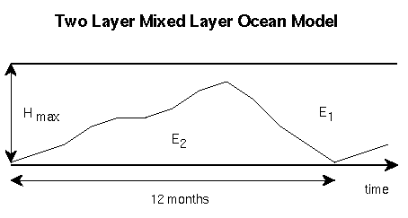
The model ocean is thermally active above the annual mixed layer maximum. It consists of an upper mixed layer, which exchanges heat with the atmosphere through radiative, latent and sensible heat fluxes, and a deeper oceanic layer, which exchanges heat with the mixed layer through entrainment and detrainment. Heat transport caused by advection and diffusion is calculated as the implied oceanic heat divergence/convergence resulting from net heat flux into the ocean when the GCM is forced by observed sea surface temperature (SST). The variation in mixed layer depth is prescribed from climatology, while the SST and heat storage between the mixed layer depth and its annual maximum is predicted by the model. Cooling of sea water at its freezing point results in formation of sea ice and possible accumulation of snow. Ice and snow thickness are prognostic variables in the thermodynamic sea ice model.

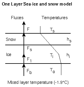
When the mixed-layer temperature reaches the freezing point for seawater (about 271 K), sea ice forms. Further cooling leads to thicker sea ice. A one-dimensional thermodynamic very similar to that of Semtner (1976) has been implemented in our model ocean. Jensen et al. (1991) presented some aspects of an early version of this combined ocean and sea ice model. The sea ice model has a single layer of ice that allows accumulation of snow on top. The model calculates an equilibrium surface temperature based on fluxes through the ice and snow as shown in the figure. Unbalanced positive fluxes into the sea ice are used to melt snow or sea ice, while cooling leads to sea ice growth.

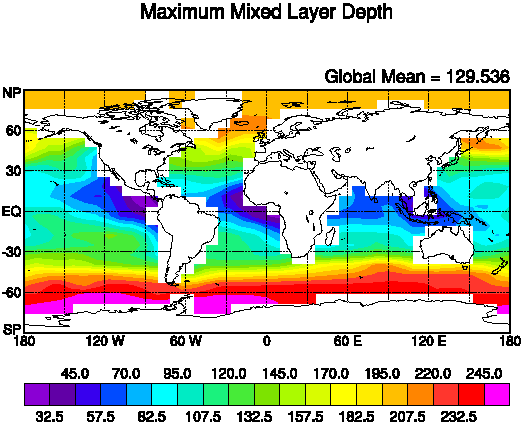
The depth of the mixed is prescribed using monthly observations. The deepest mixed layer depth during the year determines the depth of the oceanic layer which is allowed to exchange heat with the atmosphere in this model. In the real ocean, this maximum mixed layer depth varies from about 30 m in the tropics to more than 2000 m in polar regions. In the model, we only include mixed layer depth up to 255 m (deeper mixed layers are truncated to 255 m). The figure show this maximum depth. Note that the maximum depth at different locations occurs at different times during the year. At midlatitudes, the deepest mixed layer occurs in late winter.

We made an 8 year long atmospheric GCM run with climatological monthly SSTs (monthly averages computed from 1979-1988). From this control run the net downward heat flux into the ocean was computed. Using the observed SST and observed mixed layer depth, the monthly heat content in the ocean was calculated. 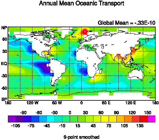From these two quantities one can calculate the implied oceanic heat divergence (Russell et al., 1985) if one assumes that the earth is in thermal equilibrium. In particular, the annual mean of the net downward heatflux has the same magnitude, but opposite sign, as the annual mean oceanic heat transport divergence. Note for instance that the ocean is a heat sink in the upwelling regions in the eastern equatorial Pacific and along eastern boundariess, while western boundary currents gives heat back to the atmosphere. Monthly fields of oceanic heat divergence was used to prescribe the oceanic heat transport for the simulations.

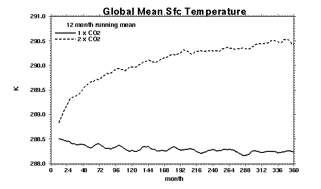
Annually and globally averaged earth surface temperature during two 30 year runs of the GCM coupled to the ocean and sea ice model. Unit are degree Kelvin. The CSU GCM predicts an increase of 2.2 K (the difference between the 1 X CO2 run and the 2 x CO2 runs) after 30 year in response to a doubling of CO2.

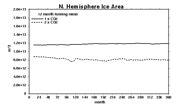
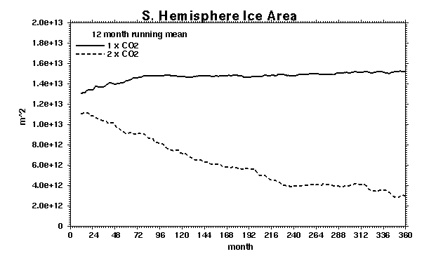
The coupled model gives a smaller sea ice area in the case of doubled CO2. In the northern hemisphere (top) the response is fast with a 30% reduction in the annual average sea ice area. Around Antartica the sea ice area is reduced every year throughout the integration (bottom). Given the rather simple sea ice model, the magnitude of these sea ice area changes may not be realistic.

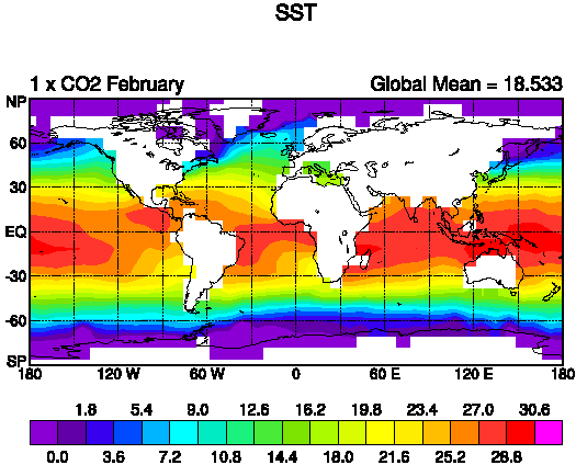
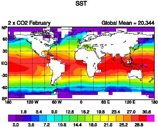
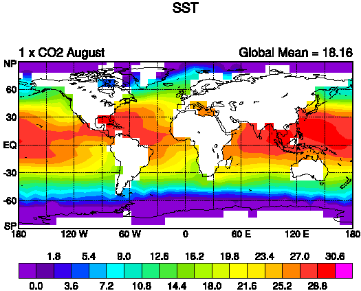
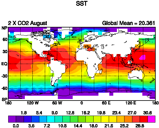
The sea surface temperature (SST) increases as a response to increased CO2. The increase in temperature is largest in polar latitudes and smallest in the tropics.

References

Jensen, T. G., D. A. Dazlich and D. A. Randall, 1995: A one-dimensional mixed layer ocean and sea ice model with prescribed oceanic heat transport. Dept. of Atmospheric Science Paper, 593, 48 pp.

Russell, G. R., J. R. Miller and L.-C. Tsang, 1985: Seasonal oceanic heat transports computed from an atmospheric model. Dyn. Atmos. Oceans, 9, 253-271.

Sellers, P. J. , L. Bounoua, G. J. Collatz, D. A. Randall, D. A. Dazlich, S. O. Los, J. A. Berry, I. Fung, C. J. Tucker, C. B. Field, and T. G. Jensen, 1996: A comparison of the radiative and physiological effects of doubled CO2 on the global climate. Science, 271, 1402-1406.

Semtner, A. J., 1976: A model for the thermodynamic growth of sea ice in numerical investigations of climate. J. Phys. Oceanogr., 6, 379-389.