Research Work Performed with the UCLA/CSU CEM

I. The cumulus ensemble model

The model used for performing the following research work is the UCLA/CSU CEM, developed by S. Krueger and A. Arakawa at UCLA. It has been modified and improved at CSU in the last few years.

CEMs are designed to simulate the formation of an ensemble of clouds that developed simultaneously and randomly inside the model domain under a given large-scale condition as if the CEM was situated with a grid box of a large-scale numerical model. Thus, information on large-scale destabilizing and moistening rates is imposed on CEM grid points uniformly in the horizontal. The methods for imposing large-scale forcings are identical to those used in Single-column Models (SCMs). See Randall et al. (1996) for further discussion.

The major difference between an SCM and a CEM is that cloud-scale circulations are explicitly resolved in a CEM, but must be parameterized in an SCM. CEMs can simulate bulk cloud properties such as cloud fraction and condensate mixing ratio, which are not reliably observed. Moreover, the simulated variables associated with the statistical properties of the clouds are internally consistent. On the other hand, CEMs do not explicitly resolve every scale of motions; they must have finer-scale parameterizations such as turbulence closure, cloud microphysics and radiative transfer. CEMs have additional limitations, for example, the periodic lateral-boundary conditions. These limitations may or may not impact the simulated cloud-scale processes that have to be parameterized in an SCM. Thus, CEMs can be used as a valuable or complementary tool for SCMs to achieve the goal of improving cloud parameterizations in GCMs or numerical weather prediction models (Browning 1994; Randall et al. 1996).

A concise description of the UCLA/CSU CEM is as follows. A detailed description can be found in Krueger (1988), Xu and Krueger (1991), Krueger et al. (1995), and Xu and Randall (1995a).

Fig. 1: A concise description of the UCLA/CSU CEM.

References:
Browning, K. A., 1994:
GEWEX cloud system study (GCSS) science plan. IGPO Publication Series, No. 11, International GEWEX Project Office, 84 pp.
Harshvardhan, R. Davies, D. A. Randall, and T. G. Corsetti, 1987:
A fast radiation parameterization for general circulation models. J. Geophys. Res., 92, 1009-1016.
Kessler, E., 1969:
On the Distribution and Continuity of Water Substance in Atmospheric Circulations. Meteor. Monogr. No. 32, Amer. Meteor. Soc., 84 pp.
Krueger, S. K., 1988:
Numerical simulation of tropical cumulus clouds and their interaction with the subcloud layer. J. Atmos. Sci., 45, 2221-2250.

Krueger, S. K., Q. Fu, K. N. Liou, and H.-N. Chin, 1995:
Improvements of an ice-phase microphysics parameterization for use in numerical simulations of tropical convection. J. Appl. Metero., 34, 281-287.
Lord, S. J., H. E. Willoughby, and J. M. Piotrowicz, 1984:
Role of a parameterized ice-phase microphysics in an axisymmetric, nonhyologic tropical cyclone model. J. Atmos. Sci., 41, 2836-2848.
Randall, Xu, Somerville and Iacobellis, 1996:
Single-column models and cloud ensemble models as links between observations and climate models.
Journal of Climate, 9, 1683-1697.
Xu and Krueger, 1991:
Evaluation of cloudiness parameterizations using a cumulus ensemble model.
Monthly Weather Review, 119, 342-367.
Xu and Randall 1995a:
Impact of interactive radiative transfer on the macroscopic behavior of cumulus ensembles. Part I: Radiation parameterization and sensitivity tests. J. Atmos. Sci., 52, 785-799.

II. Simulations of the July 1995 ARM IOP

The following describes some results from simulations of cumulus ensembles at the Southern Great Plains during the July 1995 Intensive Observation Period (IOP) of the Atmospheric Radiation Measurement (ARM) program. A detailed comparison with available observations is made. In general, the CEM simulated results agree reasonably well with the available observations from the July 1995 IOP. The differences between simulations and observations are, however, much larger than those obtained in tropical cases, especially those based on the GARP Atlantic Tropical Experiment Phase III data. The radiative budgets and satellite-observed cloud amounts are also compared with observations. Although the agreements are reasonably good, some deficiencies of the model and inadequate accuracy of large-scale advective tendencies can be clearly seen from the comparisons. Sensitivity simulations are performed to address some of these uncertainties.

Main figures related to the simulations are presented in the following paragraphs [see Xu and Randall (1999) for details].

a. The imposed large-scale forcings

The July 1995 IOP covers an 18-day period, starting from 0000 UTC on 18 July and ending at 2300 UTC on 4 August. Balloon-borne soundings of winds, temperature and dewpoint temperature are obtained every 3 h from the cloud and radiation testbed (CART) central facility located near Lamont, OK (36.61 N, 97.49 W) and from four boundary facilities, which form a rectangle of approximate 300 km x 370km. Hourly wind data from 17 profilers surrounding the CART array are also available as additional inputs for the constrained variational objective analysis performed by M.-H. Zhang (see Zhang and Lin 1997). This analysis provides a dynamically and thermodynamically consistent data set in terms of vertically integrated quantities, with adjustments not far exceeding the uncertainties of the original measurements.

All surface constraint variables are first gridded and then areally averaged. Measurements from a variety of platforms such as the sondes, surface meteorological observation system (SMOS), energy balance/Bowen ratio (EBBR), and Oklahoma (OK) Mesonet and Kansas Mesonet were merged to produce the surface composites for the constrained variational analysis. There are two versions of analyses performed by M.-H. Zhang, one with the EBBR surface fluxes and the other with the SiB2 surface fluxes. In Figs. 2 and 3, only the SiB2 fluxes-based analysis is shown.

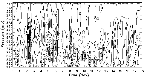
Fig. 2: Time-height cross section of the observed total advective tendency of temperature for the July 1995 IOP. The contour interval is 5 K/day.

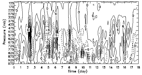
Fig. 3: Time-height cross section of the observed total advective tendency of specific humidity for the July 1995 IOP. The contour interval is 6 g/kg/day.

b. Comparison with selected observations

A series of simulations have been performed with the CEM as a part of the ARM SCM intercomparison study (Ghan et al. 1999), which compares the performance of various SCMs and a two-dimensional (2-D) CEM with ARM IOP data sets by providing a common set of forcing data and supporting data for running the SCMs and CEMs. The goal of the intercomparison study is to identify the data requirements for the ARM SCM research and to facilitate scientific advances by promoting collaborations among ARM Science Team members through common activities; specifically, to improve the representations of cloud formative/dissipative processes in GCMs and their interactions with radiation.

The baseline simulation for the intercomparion study is D2, which uses the total advective forcing shown in Figs. 2 and 3. Simulation D shown below is identical to D2 except for using the EBBR fluxes-based analysis. The advective forcings are only slightly different between the two versions of the analyses. The surface fluxes prescribed in the model are, however, drastically different during daytime (Doran et al. 1998). In addition, the horizontal inhomogeneity of the surface fluxes is allowed in the CEM.

The following figures (Figs. 4-8 and 10) indicates that the simulated results compare favorably with the selected observations although the simulated temperature and moisture biases are higher than those for tropical cases. The baseline simulation D2 is slightly superior than D in the time series of precipitable water and the vertical profile of temperature (Fig. 10a).

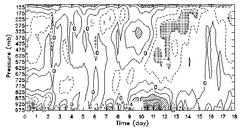
Fig. 4: Time-height cross section of the simulated temperature differences from observations for simulation D2. The contour interval is 2 K. Contours over 4 K are hatched. Contours less than -4 K are dotted.

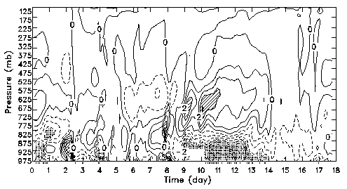
Fig. 5: Time-height cross section of the simulated moisture differences from observations for simulation D2. The contour interval is 1 g/kg. Contours over 3 g/kg are hatched. Contours less than -3 g/kg are dotted.

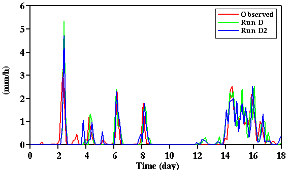
Fig. 6: Time sequences of the observed and simulated surface precipitation rates for the July 1995 IOP. Simulations D and D2 adopt the total advective forcing method; D with the EBBR fluxes and D2 with the SiB2 fluxes.

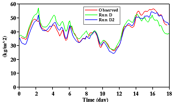
Fig. 7: Time sequences of the observed and simulated precipitable water (vertically integrated water vapor mixing ratios) for the July 1995 IOP. Simulations D and D2 adopt the total advective forcing method; D with the EBBR fluxes and D2 with the SiB2 fluxes.

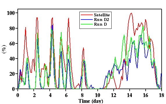
Fig. 8: Time sequences of the satellite-observed and simulated high-level cloud amounts for the July 1995 IOP. Simulations D and D2 adopt the total advective forcing method; D with the EBBR fluxes and D2 with the SiB2 fluxes.

c. EBBR vs. SiB2 fluxes

Figures 6, 7, 8, and 10 give a comparison between the two simulations with different surface fluxes. Note that the imposed large-scale forcings in these two simulations are also slightly different, as a consequence of the variational analysis. Most of the simulated results between D and D2 are similar except for the precipitable water. The precipitable water in D is generally higher in the first 14 days but lower in the last four days, compared with D2. This is related to the large differences of the SiB2 and EBBR fluxes (Fig. 9). These differences also impact the simulated temperature and moisture biases (Fig. 10).

Based upon the intercomparison study (Ghan et al. 1999), the differences in results between EBBR and SiB2 fluxes are much smaller than those between the different forcing methods. Another question yet to be answered is how much diferences are due to the surface fluxes and how much differences are due to the changes in the large-scale forcings. The large RMS temperature differences in the upper troposphere (Figs. 10a and 10b) suggests that the changes in the large-scale forcings do impact the results.

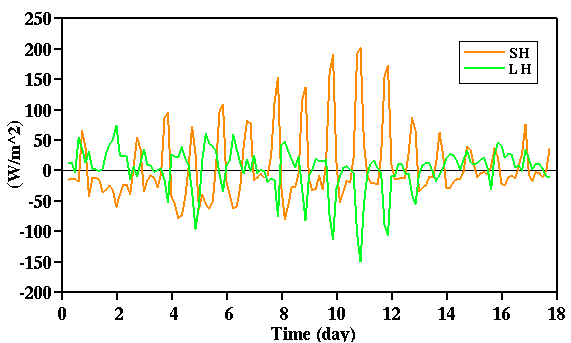
Fig. 9: Time sequence of the differences of sensible heat (SH) fluxes and latent heat (LH) fluxes between SiB2 derived and EBBR observed data.

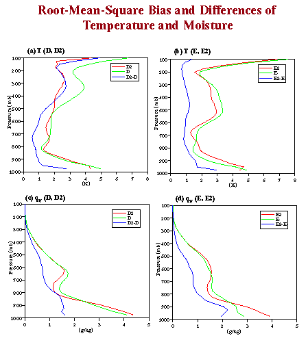
Fig. 10: Vertical profiles of root-mean-square (RMS) errors/bias from the observations and the RMS differences between D and D2 (between E and E2) for temperature (a and b) and specific humidity (c and d). Simulations E and E2 are respectively identical to D and D2 except with the vertical advective forcing method.

d. Vertical advective forcing vs. total advective forcing methods

There are at least three methods for imposing the large-scale advective forcings in a CEM or an SCM; i.e., the total advective forcing, the vertical flux forcing, and the nudging methods. The vertical advective forcing method uses the large-scale vertical velocity and horizontal temperature and moisture advections. Li et al. (1999) found that the vertical flux forcing method produced smaller biases than the total advective forcing method with the TOGA COARE data set, presumably due to the adjustment of vertical thermodynamic structure to the imposed large-scale vertical velocity, especially in the temperature profiles. Such a conclusion is further tested with the ARM data set here.

Simulations E and E2 shown in Fig. 10 are respectively identical to D and D2 except for adopting the vertical advective forcing method. Figure 11 and 12 show the time-height cross sections of temperature and moisture differences between simulations E2 and D2. The different methods do impact the results, i.e., in the vertical profiles and temporal evolutions of temperature and moisture (in the lower troposphere only).

Which method produces better results? It depends upon the subperiods in the simulation. Take the 18-day simulation as a whole, the answer can be found in Fig. 10 by judging the magnitudes of the RMS biases. For the runs with the SiB2 fluxes, simulation D2 is slightly better, while simulation E is slightly better for the runs with the EBBR fluxes. Thus, Li et al.'s conclusion is dependent upon the quality of the given data set. If the forcing data is very accurate, the total advective forcing method is superior as far as the UCLA/CSU CEM is concerned.

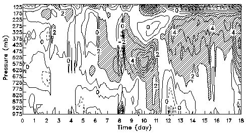
Fig. 11: Time-height cross section of the temperature differences between simulations E2 and D2. The contour interval is 2 K. Contours over 2 K are hatched. Contours less than -2 K are dotted.

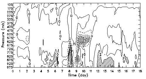
Fig. 12: Time-height cross section of the moisture differences between simulations E2 and D2. The contour interval is 1 g/kg. Contours over 2 g/kg are hatched. Contours less than -2 g/kg are dotted.

e. LLNL vs. SUNY forcings

Two very different methods were used to analyze the July 1995 IOP data set. One was performed at LLNL (Leach, Cederall et al. 1999) and the other was performed at SUNY (Zhang and Li 1987). The latter has been adopted as the standard method for the ARM SCM intercomparison study. Figure 13 shows the 18-day mean and standard deviation of the temperature and specific humidity total advective tendencies as analyzed at LLNL and at SUNY. The LLNL analysis only adopted the Barnes' (1964) objective method without the constraints used in the variational analysis. The temperature tendency shows a good agreement between the two analyses except for smaller cooling between 850 and 375 mb. On the other hand, the moisture tendency of the LLNL analysis shows much larger temporal variations and noticeably complicated vertical structures in both the mean and standard deviation profiles. Another noticeable difference is the presence of much higher warming and drying rates below 500 km. This could impact the simulated results.

The differences in the simulated results using the LLNL and SUNY forcings are apparently larger than those due to forcing methods or the surface fluxes shown above. The surface precipitation rate is only well reproduced at the end of the IOP with the LLNL forcing (Fig. 14). The precipitable water is well underestimated during the IOP (Fig. 15). This result is related to the much larger advective drying in the lower troposphere of the LLNL forcing (Fig. 13b).

On the other hand, a surprising strength of the LLNL analysis is that more abundant upper-level clouds are produced in spite of weak intensity of surface precipitation so that the OLR agrees with satellite observations rather well (Fig. 16). This is related to the similarity in the forcing data in the upper troposphere (Fig. 13). The lack of surface precipitation is due to the fact that the drier atmosphere does not allow rainwater to reach the ground due to evaporation.

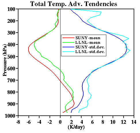
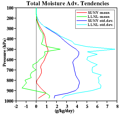
Fig. 13: Vertical profiles of the mean and standard deviations of the large-scale advective tendencies for temperature and specific humidity for both LLNL and SUNY data sets.

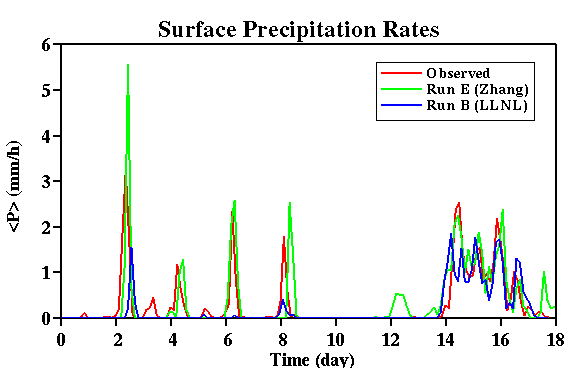
Fig. 14: Time sequence of the observed and simulated surface precipitation rates for the July 1995 IOP. Simulations B and E adopt the vertical advective forcing method; B with the LLNL data set and E with the SUNY (Zhang) forcing. Both were performed with the EBBR fluxes.

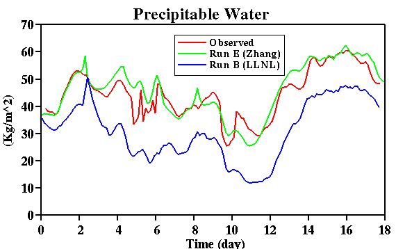
Fig. 15: Time sequence of the observed and simulated precipitable water (vertically integrated water vapor mixing ratios) for the July 1995 IOP. Simulations B and E adopt the vertical advective forcing method; B with the LLNL data set and E with the SUNY (Zhang) forcing. Both were performed with the EBBR fluxes.

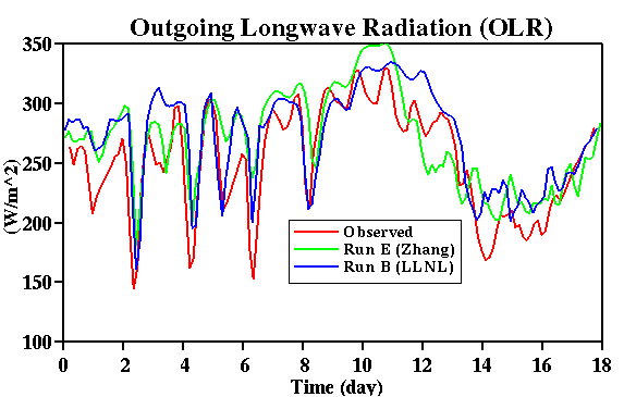
Fig. 16: Time sequence of the observed and simulated outgoing longwave radiation (OLR) fluxes for the July 1995 IOP. Simulations B and E adopt the vertical advective forcing method; B with the LLNL data set and E with the SUNY (Zhang) forcing. Both were performed with the EBBR fluxes.

References:
Barnes, S. K., 1964:
A technique for maximizing details in numerical weather map analysis. J. Appl. Meteor., 3, 396-409.
Doran, J. C., J. M. Hubbe, J. C. Liljegren, W. J. Shaw, G. J. Collatz, D. R. Cook, and R. L. Hart, 1998.
A technique for determining the spatial and temporal distributions of surface fluxes of heat and moisture over the southern great plains cloud and radiation testbed. J. Geophys. Res., 103, 6109-6121.
Ghan, S., and 19 coauthors, 1999:
An intercomparison of single column model simulations of summertime midlatitude continental convection. J. Geophys. Res., (to be submitted).
Leach, M., R. Cederwall, etc. 1999:
Objective anaylsis of ARM SCM IOP data sets (to be submitted).
Li, X., C.-H. Sui, K.-M. Lau, and M.-D. Chou, 1999:
Large-scale forcing and cloud-radiation interaction in the tropical deep convective regime. J. Atmos. Sci., (in press).
Xu, and Randall, 1999:
Explicit simulation of midlatitude cumulus ensembles. Part I: Comparison with ARM data. J. Atmos. Sci., (submitted).
Zhang, M. H., and J. L. Lin, 1997:
Constrained variational analysis of sounding data based on column-integrated budgets of mass, heat, moisture, and momentum: Approach and application to ARM measurements. J. Atmos. Sci., 54, 1503-1524.

III. Simulations of tropical oceanic convection

a. GATE Phase III

Description of GATE simulations and available CEM data for SCM validations

b. TOGA COARE

GCSS WG4 Intercomparison Study: Case 2

c. Sensitivity to initial condition and forcing data

The GATE simulation was performed with slightly altered initial conditions. An ensemble average of three simulations was used to represent the simulated results. From Figs. 17 and 18, both temperature and specific humidity deviations from the ensemble average can be much higher than the initial purturbations. The timing of the occurrence of mesoscale systems can be related to the large amplitudes of the deviations, for example, around day 12 (12 September 1974). Another point worth mentioning is that the temperature and specific humidity deviations of the unperturbed run is not always the smallest among the three runs. Thus, an ensemble of simulations, instead of a single simulation, are needed to obtain the best results for a given large-scale forcing data set.

The TOGA COARE analysis performed at SUNY with the variational analysis is used for studying the sensitivities to the initial condition and the large-scale forcing. Three versions of the analysis are available, with slightly different constrained data.

All simulations start from 18 Z December 18 1992, using the total advective forcing method. For each version of the data set, three different initital conditions are used, as in the GATE simulation. The results shown in Figs. 19, 20 (precipitable water) and 21 (surface precipitation rate) indicate that the results are more sensitive to the initial conditions than to the imposed large-scale forcings. Remember that precipitable water is a vertically integrated quantity. The differences between the purturbation runs are as large as those between simulation and observation. Those between different versions of the data set are smaller (Fig. 20). Again, this suggest that the ensemble simulations are needed to obtain representative results for a given large-scale forcing data set.

The larger sensitivity to the initial condition is probably related to the coare temporal resolution of the TOGA COARE data set (6 h vs. 3 h in GATE). That is, a comparison of temporal variations from a single simulation with observations is probably more misleading with the TOGA COARE data set than the GATE data set.

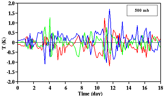
Fig. 17: Time sequences of temperature deviations at 500 mb from the ensemble average for each simulation in the ensemble using the GATE Phase III data.

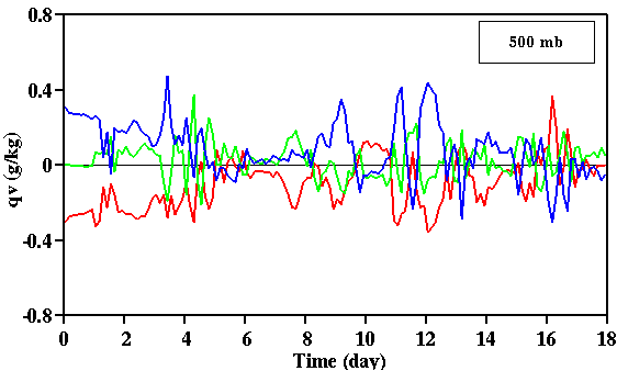
Fig. 18: Time sequences of specific humidity deviations at 500 mb from the ensemble average for each simulation in the ensemble using the GATE Phase III data.

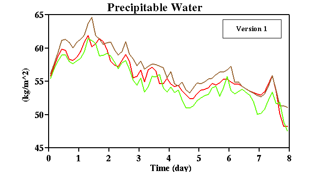
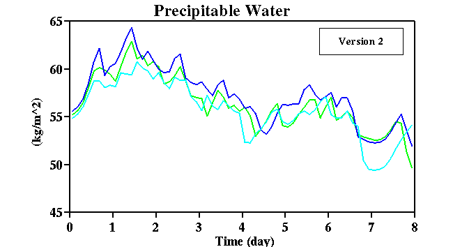
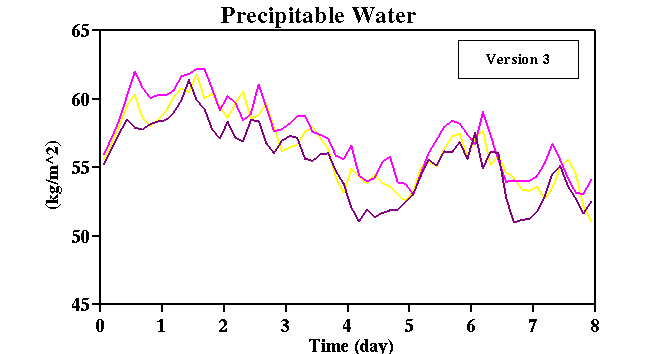
Fig. 19: Time sequences of precipitable water for each perturbed simulation with three different versions of the TOGA COARE data set, starting from 18Z, December 18 1992. Three simulations were performed for each version of the forcing data.

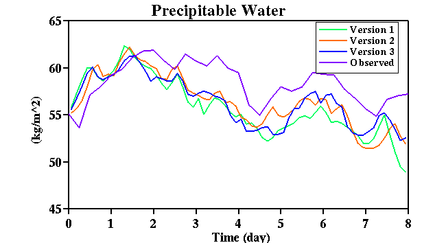
Fig. 20: Time sequences of ensemble averaged precipitable water for each version of the TOGA COARE data set, as well as that of the observation.

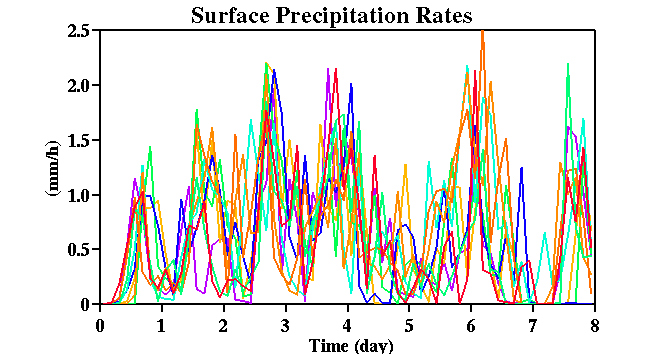
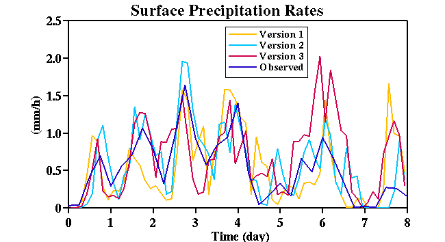
Fig. 21: Time sequences of surface precipitation rates for all simulations and the ensemble average for each version of the data set. The observed precipitation rate is also shown in the bottom panel.

IV. Comparison of statistical properties of midlatitude continetal with tropical oceanic convection

Significant differences exist between the statistical properties of tropical and midlatitude cumulus convection, especially in the vertical structures of the cumulus mass fluxes, apparent heat source (Q1) and apparent moisture sink (Q2). The strong variations of the subcloud-layer thermodynamic structure and the surface fluxes in midlatitude continents have large impacts on the heat and moisture budgets.

Figure 22 shows the mean profiles of the heat and moisture budget components over 18-day for ARM (simulation D2) and GATE (simulation G) data set. Significant differences between the two simulations appear in the condensation and evaporation rates. The condensation rate is much smaller in midlatitudes than in the Tropics, due to smaller amounts of shallow clouds. The evaporation rates are more comparable, in spite of the drier midlatitude atmosphere, because in-cloud evaporation in D2 is rather small.

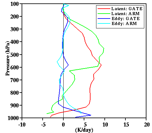
Fig. 22a: Vertical profiles of the latent heat release and the convergence of eddy heat fluxes for the 18-day mean of simulation D2 (ARM) and G (GATE).

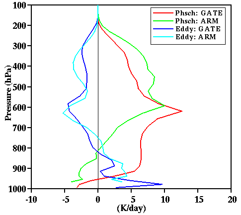
Fig. 22b: Vertical profiles of the phase change rate and the convergence of eddy moisture fluxes for the 18-day mean of simulations D2 (ARM) and G (GATE).

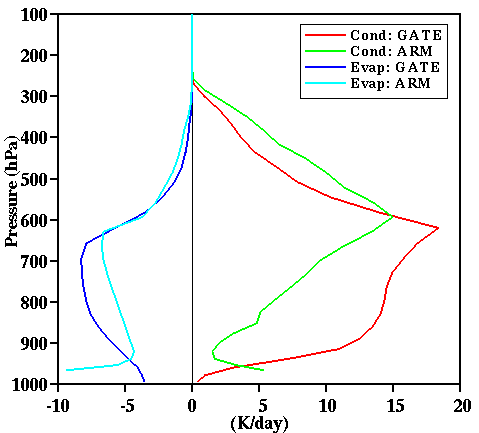
Fig. 22c: Vertical profiles of the condensation and evaporation rates for the 18-day mean of simulations D2 (ARM) and G (GATE).

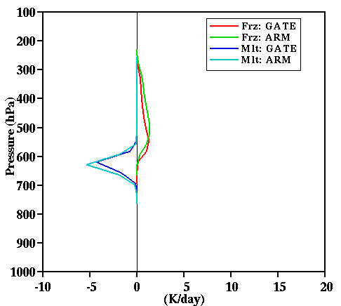
Fig. 22d: Vertical profiles of the freezing and melting rates for the 18-day mean of simulations D2 (ARM) and G (GATE).

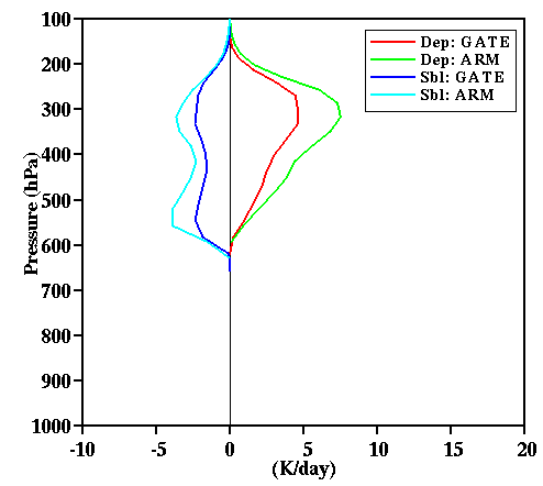
Fig. 22d: Vertical profiles of the deposition and sublimation rates for the 18-day mean of simulations D2 (ARM) and G (GATE).

Another type of comparison between midlatitude continental and tropical oceanic convection is performed with the draft statistics approach as in aircraft meansurement studies (LeMone and Zipser 1980; Jorgensen et al. 1985; Jorgensen and LeMone 1989; Lucas et al. 1994; Wei et al. 1998). Aircraft observations of cumulus drafts revealed the statistical behavior of updraft and downdraft vertical velocity. Some recent observations also provided some information on the buoyancy of updrafts and downdrafts.

The sign of buoyancy is important for determining whether or not the updraft (downdraft) is accelerating or decelerating. Observations of Jorgensen and LeMone (1989), Lucas et al. (1994) and Wei et al. (1998) showed that downdrafts with positive buoyancy and updrafts with negative buoyancy commonly occur, suggesting that decelerating drafts occur almost as commonly as accelerating drafts.

Draft statistics from cloud-resolving simulations of tropical and midlatitude cumulus convection are examined, following the procedure used in observations. Only the drafts with absolute vertical velocities exceeding 1 m/s are included in the statistics. Statistics of vertical velocity, buoyancy with/without loading effects, liquid static energy, total water mixing ratio, condensate mixing ratio are provided.

In general, we find that the medium values of updraft/downdraft strengths and other properties show the greatest similarity between tropical and midlatitude cumulus convection. The strongest 10% of midlatitude drafts are different from their counterparts in the Tropics (Fig. 23), with much stronger downdrafts and updrafts in the midlatitudes. The greatest differences in the statistics of thermodynamic properties of midlatitude and tropical cumulus convection occur in the lower troposphere, due to the much drier environments of the continental convection (Figs. 23, 24 and 25).

Fig. 23: Vertical profiles of the medium (50 percentile) and 90 percentile of updraft and downdraft vertical velocity. Solid lines are for the ARM simulations and the dashed lines for the GATE simulations.

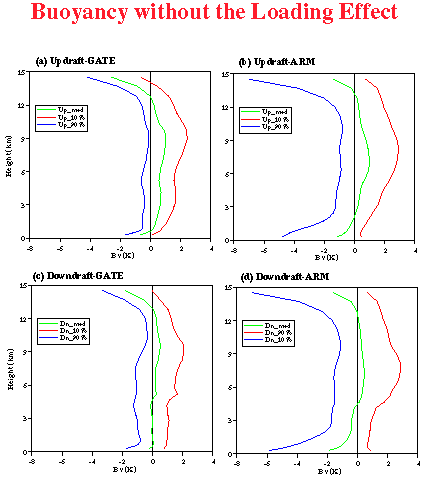
Fig. 24: Vertical profiles of the medium (50 percentile), 10 percentile and 90 percentile of updraft and downdraft buoyancy for both ARM and GATE simulations.

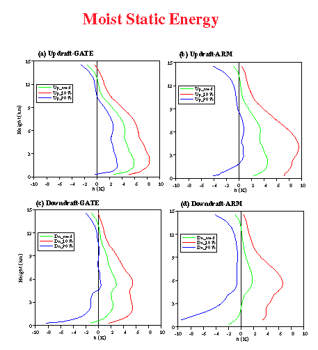
Fig. 24: Vertical profiles of the medium (50 percentile), 10 percentile and 90 percentile of updraft and downdraft moist static energy for both ARM and GATE simulations.

References:
Jorgensen, D. P., and M. A. LeMone, 1989:
Vertical velocity characteristics of oceanic convection. J. Atmos. Sci., 46, 621-640.
Jorgensen, D. P., E. J. Zipser, and M. A. LeMone, 1985:
Vertical motions in internse hurricanes. J. Atmos. Sci., 42, 839-856.
LeMone, M. A., and E. J. Zipser, 1980:
Cumulonimbus vertical velocity events in GATE. Part I: Diameter, intensity and mass flux. J. Atmos. Sci., 37, 2444-2457.
Lucas, C., E. J. Zipser, and M. A. LeMone, 1994:
Vertical velocity off Tropical Australia. J. Atmos. Sci., 51, 3183-3193.
Wei, D., A. M. Blyth, and D. J. Raymond, 1998:
Buoyancy of convective clouds in TOGA COARE. J. Atmos. Sci., 55, 3381-3391.

V. Radiative-convective equilibrium simulations

The details of this type of simulations were given at Xu and Randall (1999).